This post is the first of many that will demonstrate the difference between the taxable and assessed values in communities throughout Southeastern Michigan and explain the various taxes levied in these communities and their use. We will highlight at least one community in each county in the region and this post discusses Eastpointe in Macomb County. Eastpointe, formerly known as East Detroit, has a population of about 32,000, a median income of about $46,000 and a median home value of $64,700, according to the U.S. Census Bureau.

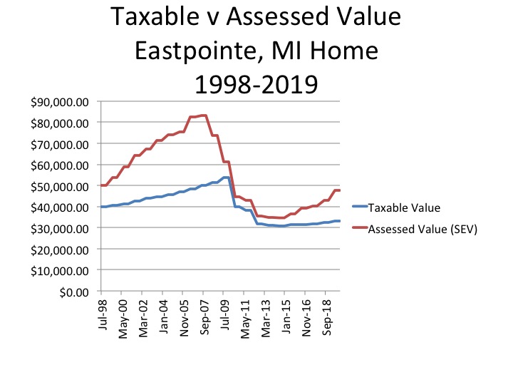
The chart below shows the taxable value and assessed value of a hypothetical Eastpointe home, beginning in July of 1998 through December of 2019. The taxable value is the value used to calculate a property’s taxes, and each year it can only increase by 5 percent or the rate of inflation, whichever is less. This number may be equal to the property’s state equalized, or assessed value, but not more than those values. Such limits on tax growth, or lack thereof, is a result of Proposal A, a state constitutional amendment approved by voter referendum in 1994. The assessed value of a property, or the state equalized valued (SEV), is usually about half of a property’s true cash value, and the true cash value is the fair market value of the property.

In 1998 the taxable value of the Eastpointe property examined was $40,000 and the assessed value was $50,000. In July of 2007 the assessed value of the property peaked at $83,252 but the taxable value was only at $50,186. By 2008 the Great Recession hit Southeastern Michigan and both the assessed values and taxable values of properties began to decline. Between July of 2007 and July of 2010 the assessed value decreased from $83,252 to $40,700, or more than 50 percent ($40,000). The annual declines continued after the recession, and the assessed value of the property reached its lowest point in July of 2014 at $34,641, a nearly 60% decline from its peak. Since July of 2014 the assessed value of the property has increased to $47,840.

As noted, the taxable value of the property was $40,000 in July of 1998, but it did not increase nearly as much as the assessed value did, because it cannot rise more than the rate of inflation or 5 percent from year-to-year. As a result, the taxable value of the property did not peak until July of 2009 ($53,599). A year later though, in July of 2010, the taxable value plummeted to $39,749. A property’s taxable value can decrease in such a way if there is a physical loss to the property and/or if the property is sold in the previous tax year. The Great Recession began in 2008 and by 2010 the taxable value of properties were on the decline, ultimately affecting governmental budgets, and services. In July of 2013 the taxable value of this Eastpointe property reached its low point at $30,804. Since then the taxable value of the property has only increased to $33,095.

Due to economic trends and the way taxable values and assessed values are calculated under Proposal A of, the assessed value of a property is nearly always higher than the taxable value. For this specific property, the only time the taxable value and assessed value were nearly the same was in July of 2009, when the taxable value was $39,749 and the assessed value was $40,700. In addition, while the gap between the two values has not been nearly as large as it was prior to the recession, since 2016 that gap has been widening.

As noted earlier, our various forms of government rely on property taxes to function, primarily our local governments (municipalities and school districts). The chart above shows that just because the local economy is recovering since the Great Recession, the budgets of local governments are not necessarily reaping the benefits. According to a recent report by the Michigan Municipal League, 173 cities in Michigan have experienced a 2 percent or less revenue growth in the last 15 years and an additional 52 have experienced a budget growth of 3 percent or more. For Eastpointe, according to the a recent report released by the Michigan Municipal League, the total revenue for the city in 2002 was $22.3 million, and in 2017 it was $25.8 million. While the total revenue for Eastpointe has increased by 16 percent the revenue generated by property and income taxes declined by 23 percent. However, while the effects of limited property tax have negatively affected municipalities across the state, the slow growth of such taxes has benefitted for the property owners. According to a September 2018 Detroit Free Press article while income growth in the state has increased since the last recession, household incomes prior to the recession have not yet been recouped. Since incomes are also recovering at a slower rate, it can be viewed that the slow growth rate of property tax revenue is allowing property owners to better stay afloat economically.

It should be noted though that a, at least in Southeastern Michigan, local tax bills have become gradually more complicated as voters approve additional tax levies, to help make up for the loss in revenue as a result of the recession, and the loss in revenue due to the limited growth of taxable values. Next week we will examine the various taxes levied for this hypothetical Eastpointe property, including what they are for, what additional ones have been added over time and how the overall tax amount for the property has either increased, or decreased, over time.